Magnetization Transfer

MR voxels often contain complex microstructure with multiple different components or pools, each with unique relaxation properties. It is possible for magnetization to be transferred between these pools via several mechanisms, such as exchange of individual protons or entire molecules, or simple dipolar coupling from molecules that are in close proximity. These mechanisms can be studied in the related fields of Magnetization Transfer (MT) and Chemical Exchange Saturation Transfer (CEST). QUIT contains tools for quantitative MT (qi qmt, qi ssfp_emt), CEST (qi zspec_interp, qi lorentzian) and also for processing MPM data (qi mtsat). Example nipype workflows for CEST analysis are also provided.

• qi lineshape

• qi lorentzian

• qi mtr

• qi mtsat

• qi ssfp_emt

• qi qmt

• qi zspec_b1

• qi zspec_interp

qi lineshape

A utility to sample lineshapes and write them out to files, which can then be read by qi qmt and interpolated values used instead of calculating the lineshape during fitting. This is used principally to speed up fitting the Super-Lorentzian lineshape, which takes a long time to calculate but is smoothly valued, so can be accurately approximated using interpolation.

Example Command Line

qi lineshape --lineshape=SuperLorentzian --frq_start=500 --frq_space=500 --frq_count=150 superlorentz.json

The output will be written to the file specified on the command-line (in this case superlorentz.json).

Important Options

• --lineshape, -l

  Choose from a Gaussian, a Lorentzian or the Super-Lorentzian. Default is Gaussian.

• --T2b, -t

  Specify the nominal T2 of the lineshape. During fitting in qi qmt scaling will be used to find the actual value. Should be specified in seconds. Default is 10e-6 (10 us).

• --frq_count, -n

  Number of frequency samples. Default is 10.

• --frq_start, -s

  First saturation frequency, in Hertz. Default is 1000.

• --frq_space, -p

  Spacing of frequencies, in Hertz. Default is 1000.

qi qmt

Calculates Quantitative Magnetization Transfer parameters using the Ramani model from steady-state gradient-echo data acquired with multiple off-resonance saturation pulses.

Example Command Line

qi qmt MTSatData.nii.gz --T1=T1.nii.gz --mask brain_mask.nii.gz --lineshape=superlorentz.json --B1=B1_map.nii.gz --f0=B0_map.nii.gz --json=input.json

Note that the T1 map argument is required input to stabilise the fitting.

Example JSON File

{
    "MTSat" : {
        "TR": 0.055,
        "Trf": 0.015,
        "FA": 5,
        "sat_f0": [56360, 47180, 12060, 1000, 1000, 2750, 2770, 2790, 2890, 1000, 1000],
        "sat_angle": [332, 628, 628, 332, 333, 628, 628, 628, 628, 628, 628],
        "pulse": { "name": "Gauss", "bandwidth": 100, "p1": 0.416, "p2": 0.295 }
    }
}

Trf is the pulse-width (RF Time). p1 and p2 are the ratio of the integral of \(B_1\) and \(B_1^2\) (the integrals of the pulse amplitude and the square of the pulse amplitude) to the maximum amplitude of the pulse. Both Trf and TR should be in seconds. sat_f0 is in Hertz. The bandwidth parameter is currently unused, any value will do.

Outputs

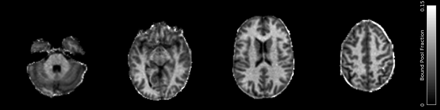
• QMT_f_b.nii.gz - The bound pool fraction

• QMT_k.nii.gz - The fundamental exchange rate between pools

• QMT_k_bf.nii.gz - The forward exchange rate from bound to free pool

• QMT_T1_f.nii.gz - T1 of the free pool

• QMT_T2_f.nii.gz - T2 of the free pool

• QMT_T2_b.nii.gz - T2 of the bound pool

• QMT_M0_f.nii.gz - The apparent Proton Density / size of the free pool

Important Options

• --R1b, -r

  Specify the relaxation rate of the bound pool. Default is 2.5 per second.

• --T1

  Path to a T1 map (in seconds). Required input to stabilise the fitting.

• --f0, -f

  Path to an off-resonance map (in Hertz).

• --B1, -b

  Path to a B1 map (ratio).

• --lineshape, -l

  Specify the lineshape to use: Gaussian, Lorentzian, Superlorentzian, or a path to a JSON lineshape file. Default is Gaussian.

• --hloss, -h

  Huber Loss parameter. Default is 1.0.

References

• Ramani et al

qi zspec_interp

Interpolates a Z-spectrum to arbitrary precision. Can output asymmetry values instead of a Z-spectrum.

Example Command Line

qi zspec_interp zspectrum.nii.gz --f0=LTZ_f0.nii.gz < input.json

The off-resonance map units must match the input frequencies (e.g. either PPM or Hertz)

Example JSON File

{
    "input_freqs" : [ -5, -2.5, 0, 2.5, 5],
    "output_freqs" : [ -5, -4, -3, -2, -1, 0, 1, 2, 3, 4, 5]
}

input_freqs are the offset frequencies the Z-spectrum was acquired at. output_freqs are the frequencies you want the asymmetry calculated at.

Outputs

• {input}_interp.nii.gz The interpolated Z-spectrum.

Important Options

• --f0, -f

  Specify an off-resonance map. Units must be the same as the input & asymmetry frequencies.

• -O, --order

  The order of Spline interpolation used. Default is 3 (cubic).

• -a, --asym

  Output asymmetry (\(Z(-f) - Z(+f)\)) values.

• --ref, -r

  Divide output by reference image and multiply by 100 to output percentages.

• --mask, -m

  Only process voxels within the specified mask.

qi zspec_b1

Corrects Z-spectra for B1 inhomogeneity using linear regression across multiple B1 levels.

Example Command Line

qi zspec_b1 b1_map.nii.gz zspec_b1level1.nii.gz zspec_b1level2.nii.gz zspec_b1level3.nii.gz < input.json

The first positional argument is a B1 map. Subsequent arguments are Z-spectrum files, one for each B1 level. The number of input files must match the length of b1_rms in the JSON.

Example JSON File

{
    "b1_rms": [1.0, 2.0, 3.0]
}

Outputs

• {input}_b1.nii.gz - The B1-corrected Z-spectrum.

Important Options

• --out, -o

  Change output suffix. Default is _b1.

• --mask, -m

  Only process voxels within the specified mask.

qi lorentzian

Fits sums of Lorentzian functions to a Z-spectrum. Highly customisable for the number of desired Lorentzian’s and their characteristics.

Example Command Line

qi lorentzian zspectrum.nii.gz < input.json

The Z-spectrum must be a 4D file with each volume acquired at a different offset frequency.

Example JSON File

{
    "MTSat": {
        "pulse": {
            "p1": 0.4,
            "p2": 0.3,
            "bandwidth": 0.39
        },
        "Trf": 0.02,
        "TR": 4,
        "FA": 5,
        "sat_f0": [0, 1, 2, 3, 4, 5],
        "sat_angle": [180, 180, 180, 180, 180, 180]
    },
    "pools" :
    [
        {
            "name": "DS",
            "df0": [0, -2.5, 2.5],
            "fwhm": [1.0, 1.e-6, 3.0],
            "A": [0.2, 1.e-3, 1.0],
            "use_bandwidth": true
        },
        {
            "name": "MT",
            "df0": [-2.5, -5.0, -0.5],
            "fwhm": [50.0, 35.0, 200.0],
            "A": [0.3, 1.e-3, 1.0]
        }
    ]
}

The input needs to include both the sequence parameters and the characteristics of the Lorentzian “pools” that you wish to fit. Currently the only important information used from the sequence are the saturation offsets, and optionally the bandwidth of the pulse. For each pool a name is required, and then triples of values representing the starting, lower and upper bound for the center frequency df0, the Full-Width Half-Maximum fwhm and amplitude A of the Lorentzian. You can also specify that the modified Lorentzian including the pulse bandwidth should be used "use_bandwidth": True. See the reference for details.

Important Options

• --pools, -p

  Number of Lorentzian pools to fit. Default is 1.

• --add, -a

  Specify an additive model instead of the default subtractive (saturation) model. Useful when a base-line has already been subtracted from the Z-spectrum. See reference for details.

• --zref, -z

  Change the reference value for the Z-spectrum. Default is 1.0, change to 0.0 for additive model.

Outputs

For each pool three outputs will be written, with an LTZ_ prefix followed by the pool name. For a single pool representing direct-saturation (DS), the following will be written:

• LTZ_DS_f0.nii.gz - The center frequency of the fitted Lorentzian.

• LTZ_DS_fwhm.nii.gz - The width of the fitted Lorentzian.

• LTZ_DS_A.nii.gz - The amplitude of the fitted Lorentzian.

References

• Deshmane et al

qi mtr

Calculates Magnetization Transfer Ratio (MTR) and related quantities, e.g. MTasym and ihMTR.

By default only the MTR is calculated, assuming that the input contains one MT-weighted and one PD-weighted (reference) volume. However it can be used to calculate other quantities by passing in a JSON file specifying the formulas to calculate these. An example is given below to calculate MTR, ihMTR and MTasym from an acquisition with five volumes which correspond to ihMTw (+/-), ihMTw (-/+), PDw, MTw (+), MTw (-) where +/- correspond to applying the saturation pulse at positive or negative frequency.

Example Command Line

qi mtr mt_volumes.nii.gz --json=contrasts.json

Example JSON File

{
  "contrasts": [
    { "name" : "MTR",    "ref": [2, 2], "add": [3, 4], "sub": [],     "reverse": true },
    { "name" : "MTasym", "ref": [2],    "add": [3],    "sub": [4],    "reverse": false },
    { "name" : "eMTR",   "ref": [2, 2], "add": [0, 1], "sub": [],     "reverse": true },
    { "name" : "ihMTR",  "ref": [2, 2], "add": [3, 4], "sub": [0, 1], "reverse": false }
  ]
}

The fields ref, add, sub refer to the indices of volumes that should be used as a reference, added or subtracted. reverse means that the contrast is reversed, i.e. it should be subtracted from the reference value before output (which is standard for MTR because it is a negative quantity). Additional supported fields are scale (a multiplicative factor, default 1.0) and inverse (boolean, default false). When inverse is true, harmonic means are used for averaging and the difference is multiplied by the reference instead of divided. An index of -1 in ref will use an external reference image specified with --ref.

Important Options

• --ref, -r

  Specify an external reference image. Can be used in contrast definitions with a ref index of -1.

Outputs

All outputs are expressed as percentages (multiplied by 100). By default there is one output:

• MTR.nii.gz - The classic MTR, expressed as a percentage

If you use a custom contrasts file then the outputs will have the names specified in the .json file.

References

1. ihMTR

qi mtsat

Implementation of Gunther Helm’s MT-Sat method. Calculates R1, apparent PD and the semi-quantitative MT-Saturation parameter “delta”. This is the fractional reduction in the longitudinal magnetization during one TR, expressed as a percentage. Arguably could be included in the Relaxometry module instead. Outputs R1 instead of T1 as this is more common in the MTSat / MPM literature. If using multi-echo input data the input should be passed through qi mpm_r2s first and the output S0 files used as input to qi mtsat. By default, does not use the original small flip angle approximation to compute R1 and PD because of the results presented in Edwards et al., 2021. To still use the small flip angle approximation (e.g., for backward compatibility), use the –smallangle (-s) flag. By default, R1 values above 10 1/s and delta values above 10% are clamped, but you can change these numbers. All delta, R1, and PD values lower than 0 are set to 0.

Example Command Line

qi mtsat PDw.nii.gz T1w.nii.gz MTw.nii.gz < input.json

Example JSON File

{
    "MTSat": {
        "TR_PDw": 0.025,
        "TR_T1w": 0.025,
        "TR_MTw": 0.028,
        "FA_PDw": 5,
        "FA_T1w": 25,
        "FA_MTw": 5
    }
}

Outputs

• MTSat_R1.nii.gz - Apparent longitudinal relaxation rate

• MTSat_PD.nii.gz - Apparent proton density / equilibrium magnetization

• MTSat_delta.nii.gz - MT-Sat parameter, see above.

Important Options

• --smallangle, -s

  If this flag is specified, use the small flip angle approximation from the original Helms et al paper. Else, do not use the approximation, as suggested in Edwards et al (default).

• --B1, -b

  Path to a B1 map (ratio).

• --C, -C

  Correction factor for delta. Default is 0.4.

• --delta-max, -d

  Clamp delta values above this value (percentage). Default is 10.

• --r1-max, -r

  Clamp R1 values above this value (per second). Default is 10.

References

• Helms et al

• Erratum

• Edwards et al <http://doi.org/10.1007/s10334-021-00947-8>

qi ssfp_emt

Due to the short TR commonly used with SSFP, at high flip-angles the sequence becomes MT weighted. It is hence possible to extract qMT parameters from SSFP data. More details will be in a forthcoming paper.

Example Command Line

qi ssfp_emt ES_G.nii.gz ES_a.nii.gz ES_b.nii.gz

Example JSON File

{
    "SSFPMT": {
        "FA": [15, 35],
        "TR": 0.005,
        "Trf": 0.002,
        "pulse": { "name": "Gauss", "bandwidth": 100, "p1": 0.416, "p2": 0.295 }
    }
}

Outputs

• EMT_T1_f.nii.gz - Longitudinal relaxation time of the free water pool

• EMT_T2_f.nii.gz - Transverse relaxation time of the free water pool

• EMT_PD.nii.gz - Apparent Proton Density

• EMT_f_b.nii.gz - Bound pool fraction

• EMT_k_bf.nii.gz - Forward exchange rate

Important Options

• --B1, -b

  Path to a B1 map (ratio).

• --G0

  Lineshape value at resonance. Default is 1.4e-5.

References

• Bieri et al

• Gloor et al