Relaxometry
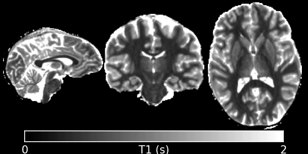
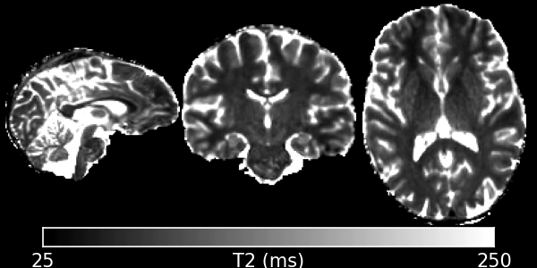
Relaxometry is the measurement of the longitudinal and transverse relaxation times T1 and T2. There are a multitude of different techniques for measuring both. The main focus of QUIT has been on the Driven-Equilibrium Single-Pulse Observation of T1 (DESPOT1) family of techniques, but the classic multi-echo T2 method and the more recent MP2RAGE T1 measurement method are also implemented. It is common for relaxometry methods to need a B1 map.
The following commands are available:
qi despot1
This command implements the classic Driven Equilibrium Single-Pulse Observation of T1 (DESPOT1) algorithm, also known as the Variable Flip-Angle (VFA) method in the literature. This is a fast way to measure longitudinal relaxation using a spoiled steady-state sequence, which is know by a different name by every scanner manufacturer just to be helpful. On GE, it’s SPoiled Gradient Recalled echo (SPGR), on Siemens it’s Fast Low-Angle SHot (FLASH) and on Phillips the sequence is Fast Field Echo (FFE).
Example Command Line
qi despot1 input_file.nii.gz --mask=mask_file.nii.gz --B1=b1_file.nii.gz < input.json
Example JSON File
{
    "SPGR": {
        "TR": 0.01,
        "FA": [3, 18]
    }
}
Outputs
D1_T1.nii.gz- The T1 map. Units are the same as those used for TR in the input.D1_PD.nii.gz- The apparent Proton Density map. No units.
Important Options
--B1, -bSpecify an effective flip-angle or B1 map. This must be expressed as a fraction, e.g. a value of 1 in a voxel implies the nominal flip-angle was achieved.
--algo, -aThis specifies which precise algorithm to use. There are 3 choices, classic linear least-squares (l), weighted linear least-squares (w), and non-linear least-squares (n). If you only have 2 flip-angles then LLS is the only meaningful choice. The other 2 choices should produce better (less noisy, more accurate) T1 maps when you have more input flip-angles. WLLS is faster than NLLS for the same number of iterations. However, modern processors are sufficiently powerful that the difference is bearable. Hence NLLS is recommended for the highest possible quality.
--its, -iMaximum iterations for WLLS/NLLS algorithms. Default is 15.
References
qi despot1hifi
This is an extension of DESPOT1 to fit a map simultaneously using an MP-RAGE / IR-SPGR type sequence. Although DESPOT1-HIFI can produce a rough estimate of B1, it often fails to produce reasonable values in the ventricles, and the fact that the MP-RAGE image is often acquired at lower resolution than the SPGR/FLASH data can also cause problems. Hence you should either smooth the B1 map produced as output, or fit it with a polynomial (Utilities), then recalculate T1 using the qi despot1 command. Note that if your MP-RAGE image is not acquired at the same resolution as your SPGR data, it must be resampled to the same spacing before processing (and it should also be registered to your SPGR data).
Example Command Line
qi despot1hifi spgr_file.nii.gz irspgr_file.nii.gz --mask=mask_file.nii.gz < input.json
Example JSON File
{
    "SPGR": {
        "TR": 0.01,
        "FA": [3, 18]
    },
    "MPRAGE": {
        "FA": 5,
        "TR": 0.01,
        "TI": 0.45,
        "TD": 0,
        "eta": 1,
        "ETL": 64,
        "k0": 0
    }
}
For the MPRAGE sequence, the TR is the spacing between readouts/echoes, not the overall segment TR. TI is the Inversion Time, and TD is the Delay Time after the echo-train (often 0). Eta is the Inversion Efficiency. Note that this value is currently hardcoded to -1.0 in the source code and the JSON value is ignored. ETL is the Echo-Train Length - usually the number of phase encode steps in one segment. k0 defines the position in the echo-train that the center line of k-space is acquired. This is 0 for centric acquisition and ETL/2 for linear.
Important Options
--clamp, -cClamp output T1 values to this value.
Outputs
HIFI_T1.nii.gz- The T1 map. Units are the same as those used for TR in the input.HIFI_PD.nii.gz- The apparent Proton Density map. No units.HIFI_B1.nii.gz- The relative flip-angle map.
References
qi despot2
DESPOT2 uses SSFP data and a separate T1 map to calculate T2, using the same maths as DESPOT1. It does not account for the banding artefacts present in SSFP data at field-strengths of 3T and above. See qi despot2fm for a method that does account for them, or if you have at least 4 phase-increments and complex data then see qi ssfp_bands in Utilities for a way to remove them before using this command.
Example Command Line
qi despot2 input_file.nii.gz --T1=t1_map.nii.gz --mask=mask_file.nii.gz --B1=b1_file.nii.gz < input.json
Example JSON File
{
    "SSFP": {
        "TR": 0.005,
        "PhaseInc": [180],
        "FA": [12, 60]
    }
}
Both PhaseInc and FA are measured in degrees. The SSFP sequence type always requires a PhaseInc entry, even when using the --gs option. The units of TR must match the input T1 map.
Outputs
D2_T2.nii.gz- The T2 map. Units are the same as those used for TR in the input.D2_PD.nii.gz- The apparent Proton Density map. No units. Will be corrected for T2 decay at the echo time.
Important Options
--B1, -bSpecify an effective flip-angle or B1 map. This must be expressed as a fraction, e.g. a value of 1 in a voxel implies the nominal flip-angle was achieved.
--algo, -aThis specifies which precise algorithm to use. There are 3 choices, classic linear least-squares (l), weighted linear least-squares (w), and non-linear least-squares (n). If you only have 2 flip-angles then LLS is the only meaningful choice. The other 2 choices should produce better (less noisy, more accurate) T1 maps when you have more input flip-angles. WLLS is faster than NLLS for the same number of iterations. However, modern processors are sufficiently powerful that the difference is bearable. Hence NLLS is recommended for the highest possible quality.
--gs, -gThis specifies that the input data is the SSFP Ellipse Geometric Solution, i.e. that multiple phase-increment data has already been combined to produce band free images. When this option is specified, the elliptical signal equation is used.
--its, -iMaximum iterations for WLLS/NLLS algorithms. Default is 15.
References
qi despot2fm
DESPOT2-FM uses SSFP data with mulitple phase-increments (also called phase-cycles or phase-cycling patterns) to produce T2 maps without banding artefacts.
Example Command Line
qi despot2fm input_file.nii.gz --T1=t1_map.nii.gz --mask=mask_file.nii.gz --B1=b1_file.nii.gz < input.json
The input file should contain all SSFP images concatenated together as a 4D file. The preferred ordering is flip-angle, then phase-increment (i.e. all flip-angles at one phase-increment, then all flip-angles at the next phase-increment).
Example JSON File
{
    "SSFP": {
        "TR": 0.005,
        "PhaseInc": [180, 180, 0, 0],
        "FA": [12, 60, 12, 60]
    }
}
Both PhaseInc and FA are measured in degrees. The length of PhaseInc and FA must match.
Outputs
FM_T2.nii.gz- The T2 map. Units are the same as those used for TR in the input.FM_PD.nii.gz- The apparent Proton Density map. No units. Will be corrected for T2 decay at the echo time.FM_f0.nii.gz- The off-resonance frequency map.
Important Options
--B1, -bSpecify an effective flip-angle or B1 map. This must be expressed as a fraction, e.g. a value of 1 in a voxel implies the nominal flip-angle was achieved.
--asym, -AWith the commonly used phase-increments of 180 and 0 degrees, due to symmetries in the SSFP magnitude profile, it is not possible to distinguish positive and negative off-resonance. Hence by default
qi despot2fmonly tries to fit for positive off-resonance frequences. If you acquire most phase-increments, e.g. 180, 0, 90 & 270, then add this switch to fit both negative and positive off-resonance frequencies.--its, -iMaximum iterations for NLLS. Default is 75.
References
qi jsr
Join-System Relaxometry fits T1 and T2 to spoiled and balanced gradient echo (SPGR and SSFP) data simultaneously, which improves the accuracy and precision in the fit of both.
Example Command Line
qi jsr spgr.nii.gz ssfp.nii.gz < input.json
Example JSON File
{
    "SPGR": {
        "TR": 0.01,
        "TE": 0.003,
        "FA": [12]
    },
    "SSFP": {
        "TR": 0.01,
        "Trf": 0.003,
        "FA": [10, 20, 20, 40],
        "PhaseInc": [180, 180, 0, 180]
    }
}
Note that the pulse-length for SSFP is required in order to apply to finite-pulse correction of Crooijmans et al. For hard-pulses this should be set to the actual length of the pulse, for other pulses an adjusted pulse-length is required as discussed in the paper.
Outputs
JSR_PD.nii.gz- The apparent Proton Density map. No units.JSR_T1.nii.gz- The T1 map. Units are the same as those used for TR in the input.JSR_T2.nii.gz- The T2 map. Units are the same as those used for TR in the input.JSR_f0.nii.gz- The off-resonance map.
Important Options
--B1, -bPath to a B1 map file.
--npsi, -pNumber of starting points for psi/off-resonance fitting. Default is 2.
References
qi mcdespot
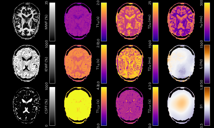
Multi-component DESPOT aims to separate SPGR and SSFP signals into multiple discrete pools with different T1 and T2. In the brain, the pool with shorter values is attributed to myelin water, while pools with longer values can be either intra/extra-cellular water or CSF.
It is recommended to have an off-resonance map to stabilise the fitting. This can be generated by using qi despot1 and then qi despot2fm above. A B1 map is also essential for good results.
Example Command Line
qi mcdespot spgr_file.nii.gz ssfp_file.nii.gz --mask=mask_file.nii.gz --B1=b1_file.nii.gz --f0=f0_file.nii.gz --scale < input.json
The SSFP input file should contain all SSFP images concatenated together as a 4D file (see qi despot2fm above).
Example JSON File
{
    "SPGR": {
        "TR": 0.01,
        "FA": [3,4,5,7,9,12,15,18],
        "TE": 0.003
    },
    "SSFP": {
        "TR": 0.05,
        "FA": [12,16,20,24,30,40,50,60,12,16,20,24,30,40,50,60],
        "PhaseInc": [180,180,180,180,180,180,180,180,0,0,0,0,0,0,0,0]
    }
}
Outputs
Note - the output prefix will change depending on the model selected (see below). The outputs listed here are for the 3 component model.
3C_T1_m.nii.gz- T1 of myelin water3C_T2_m.nii.gz- T2 of myelin water3C_T1_ie.nii.gz- T1 of intra/extra-cellular water3C_T2_ie.nii.gz- T2 of intra/extra-cellular water3C_T1_csf.nii.gz- T1 of CSF3C_T2_csf.nii.gz- T2 of CSF3C_tau_m.nii.gz- The residence time of myelin water (reciprocal of forward exchange rate)3C_f_m.nii.gz- The Myelin Water Fraction (MWF)3C_f_csf.nii.gz- The CSF Fraction3C_f0.nii.gz- The off-resonance frequency. If this was specified on the command line, it will be a copy of that file3C_B1.nii.gz- The relative flip-angle map. If this was specified on the command line, it will be a copy of that file
The intra/extra-cellular water fraction is not output, as it is not a free parameter (only 2 of the 3 pool fractions are required for the calculations). It is easy to calculate this post-hoc by subtracting the MWF and CSFF from 1.
Important Options
--SRCUse Stochastic Region Contraction (flat prior) instead of the default Gaussian Region Contraction.
--model, -M2 - 2 component model. Myelin and intra/extra-cellular water
3 - 3 component model. Myelin water, IE water & CSF
Default is 3.
--scale, -SNormalize signals to mean before fitting. Recommended.
--its, -iMaximum iterations for Region Contraction. Default is 4.
--boundsSpecify that bounds are included in the input JSON file.
References
qi mp2rage
MP2RAGE adds a second inversion time to the standard T1w MPRAGE sequence. Combining the (complex) images with the expression \(S_1 S_2^*/(|S_1^2 + S_2^2|)\) produces a real-valued image that is corrected for receive coil (B1-) inhomogeneity. In addition, if the two inversion times are carefully selected, a one-to-one mapping exists between the values in that image and T1, which is also robust to transmit (B1+) inhomogeneity. Finally, as the two images are implicitly registered, this method has several advantages over DESPOT1.
Example Command Line
qi mp2rage input_file.nii.gz < input.json
The input file must be complex-valued.
Example JSON File
{
    "MP2RAGE" : {
        "TR" : 0.006,
        "TRPrep" : 5,
        "TI" : [0.9, 2],
        "SegLength" : 128,
        "k0" : 64,
        "FA": [6, 8]
    }
}
TR is the readout or acquisition repetition time, while TRPrep is time between preparations/inversion pulses. SegLength is the number of readouts in one segment, and k0 is the index within the segment when the center line of k-space is read. This is 0 for centric order, or \(SegLength / 2\) for linear (default Siemens) order. There should be two values of TI and FA.
Outputs
MP2_UNI.nii.gz- The MP2 contrast image. The range of this image is -0.5 to 0.5.MP2_T1.nii.gz- The T1 map. Units are the same as TR and TRPrep.
Important Options
--beta, -bRegularisation factor for robust contrast calculation (see references). It is recommended to experiment with this parameter to manually find an optimum value, which should then be kept constant for an entire dataset.
References
qi multiecho
Classic monoexponential decay fitting. Can be used to fit either T2 or T2*.
Example Command Line
qi multiecho input_file.nii.gz --algo=a < input.json
Example JSON File
For regularly spaced echoes:
{
    "MultiEcho" : {
        "TR" : 2.5,
        "TE1" : 0.005,
        "ESP" : 0.005,
        "ETL" : 16
    }
}
TE1 is the first echo-time, ESP is the subsequent echo-spacing, ETL is the echo-train length.
For irregularly spaced echoes:
{
    "MultiEcho" : {
        "TR" : 2.5,
        "TE" : [0.005, 0.01, 0.03, 0.05]
    }
}
Note
The current implementation of the ARLO method will only work with regularly spaced echoes
Outputs
ME_T2.nii.gz- The T2 map. Units are the same as TE1 and ESP.ME_PD.nii.gz- The apparent proton-density map (intercept of the decay curve at TE=0)
Important Options
--algo, -al - Standard log-linear fitting
a - ARLO (see reference below)
n - Non-linear fitting
References
qi mpm_r2s
Implements the ECSTATICS method for estimating R2*, part of Multi-Parametric Mapping (MPM). This performs a simultaneous fit to PD-, T1- and MT-weighted multi-echo data for R2*, improving the SNR of the resulting fit compared to individual fits. In contrast to the original paper, which used linear least-squares, a bounded non-linear fit is used.
Example Command Line
qi mpm_r2s PDw.nii.gz T1w.nii.gz MTw.nii.gz < input.json
Example JSON File
For regularly spaced echoes:
{
    "PDw" : {
        "TR" : 2.5,
        "TE1" : 0.005,
        "ESP" : 0.005,
        "ETL" : 8
    },
    "T1w" : {
        "TR" : 2.5,
        "TE1" : 0.005,
        "ESP" : 0.005,
        "ETL" : 8
    },
    "MTw" : {
        "TR" : 2.5,
        "TE1" : 0.005,
        "ESP" : 0.005,
        "ETL" : 6
    }
}
TE1 is the first echo-time, ESP is the subsequent echo-spacing, ETL is the echo-train length.
Outputs
MPM_R2s.nii.gz- The R2* map. Same units asTE.MPM_S0_PDw.nii.gz- The PD-weighted signal atTE=0.MPM_S0_T1w.nii.gz- The T1-weighted signal atTE=0.MPM_S0_MTw.nii.gz- The MT-weighted signal atTE=0.
Important Options
--ricianSpecify the mean squared noise level for Rician noise correction. When specified, the residuals use \(data^2 - noise - signal^2\) instead of \(data - signal\). Default is 0 (no Rician correction).
References
qi ssfp_ellipse
This tool is not a relaxometry tool as such but a pre-processing step for qi planet.
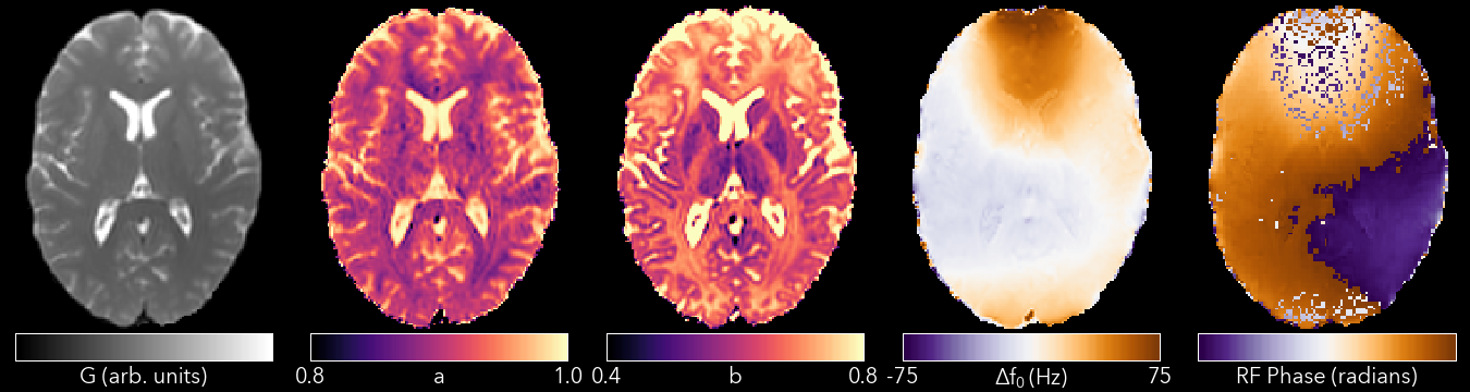
Shcherbakova et al showed it was possible to recover the ellipse parameters G, a, b from at least six phase-increments. They then proceeded to recover T1 & T2 from the ellipse parameters. This utility calculates the ellipse parameters, and qi planet then processes those parameters to calculate T1 & T2. A non-linear fit is used instead of the algebraic method used by Shcherbakova et al. This is slower, but robust across all flip-angles.
Example Command Line
qi ssfp_ellipse ssfp_data.nii.gz < input.json
The SSFP file must be complex-valued. At least three pairs of opposing phase-increments are recommended (six images in total).
Example JSON File
{
    "SSFP": {
        "TR": 0.005,
        "PhaseInc": [180, 240, 300, 0, 60, 120],
        "FA": [12, 12, 12, 12, 12, 12]
    }
}
Both PhaseInc and FA are measured in degrees. The length of PhaseInc and FA must match, but the value of FA is unused so a dummy value is permissible. If multiple ellipses with different flip-angles are present in the input data, do not specify the extra flip-angles.
Outputs
ES_G- The Geometric Solution point of the ellipse. Influences the overall size of the ellipse. This is called (M) in the Hoff and Shcherbakova papers, but it is not a measurable magnetization and hence to distinguish it a different letter is used.ES_a- The ellipse parameter that along with (G) controls the ellipse size.ES_b- The ellipse parameter that determines how flat or circular the ellipse is.ES_theta_0- The accrued phase due to off-resonance, divide by \(2\pi TE\) (or \(\pi TR\)) to find the off-resonance frequency.ES_phi_rf- The effective phase of the RF pulse.
References
qi planet
Converts the SSFP Ellipse parameters, i.e. the output of qi ssfp_ellipse, into relaxation times.
Example Command Line
qi planet ES_G.nii.gz ES_a.nii.gz ES_b.nii.gz
Example JSON File
{
    "SSFP": {
        "TR": 0.005,
        "PhaseInc": [0],
        "FA": [12]
    }
}
The length of PhaseInc and FA must match, but the value of PhaseInc is unused. There should be one value of FA for each ellipse. This means a different input file is required than for ssfp_ellipse.
Outputs
PLANET_T1.nii.gz- Longitudinal relaxation timePLANET_T2.nii.gz- Transverse relaxation timePLANET_PD.nii.gz- Apparent Proton Density
References
qi irtse
Calculates a T1 and M0 map from inversion recovery data.
Example JSON File This is an example with multiple inversion times with the same TR, 30 deg navigator flip angle.
{
    "IRTSE":
    {
        "TI":[0.1, 0.4, 0.6, 0.8, 1.0],
        "TR":[1.5, 1.5, 1.5, 1.5, 3.0],
        "Q": [-1.0, -1.0,  -1.0, -1.0, -1.0],
        "ETL": 48,
        "ESP": 0.005,
        "TD1": 0.3,
        "theta": 30
    }
}
Outputs
- IRTSE_T1.nii.gz - Longitudinal relaxation time
- IRTSE_PD.nii.gz - Apparent Proton Density
References - Padormo, F. et al.